Natural Language Processing Summarization: Extraction

Identifying which sentences are most important with PyTorch.

Introduction

Text summarization is a natural language processing task of taking long form documents and condensing them in two or three sentences. In this post, I’ll introduce a multi-step text summarization approach based off of this research paper by Chen and Bansal. Following the approach from the paper, the general approach is as follows:

1. Select sentences for extraction
2. Create abstract summaries from extracted sentences
3. Use reinforcement learning to improve extraction and abstraction

I like this approach for several reasons:

• It has a high level of intuition and is similar to how I would summarize articles. I would usually find important parts of the article (extraction) and try to put them into my own words (abstraction).
• The approach is relatively modular. The extraction and abstraction steps can be trained independently from each other.
• It uses reinforcement learning which an area of interest for me
• The original paper’s authors have provided code that I could refer to if I didn’t understand anything mentioned in the paper.

In this particular post, we will go into detail regarding my implementation of the extraction step. In future posts I will cover the abstraction and reinforcement learning steps. For now, let’s get a better idea as to how this approach works.

Problem Formulation

Ultimately, we want to create abstraction summarizations of news articles. For example we would want to turn this:

( cnn ) share , and your gift will be multiplied . that may sound like an esoteric adage , but when zully broussard selflessly decided to give one of her kidneys to a stranger , her generosity paired up with big data . it resulted in six patients receiving transplants . that surprised and wowed her . “ i thought i was going to help this one person who i don’t know , but the fact that so many people can have a life extension , that ‘s pretty big , “ broussard told cnn affiliate kgo . she may feel guided in her generosity by a higher power . “ thanks for all the support and prayers , “ a comment on a facebook page in her name read….

Into this:

zully broussard decided to give a kidney to a stranger . a new computer program helped her donation spur transplants for six kidney patients .

To accomplish this, as mentioned above, our strategy is to first extract important sentences from the original document.

Dataset

The dataset I used to train the summarization model originates from the CNN/Daily Mail summarization dataset. This dataset provides labels for 300k news articles in the form of 2-5 sentence summarizations provided by human labelers.

Although the dataset provides most of what is needed to learn extraction, the labels are not immediately useful as they are abstract summarizations produced by humans. The labels do not explicitly label which sentences are most important. In order to learn which sentences to extract, we must first produce “pseudo labelled” data. We can accomplish this by calculating which sentences of the original article have the highest ROUGE-L score with the abstract sentence summary sentences. Ultimately, our dataset looks like a list of dictionaries of the form:

[
    {
         'document': '( cnn ) share, and your gift ...', 
         'summary': 'zully broussard decided ...',
         'extraction_label': torch.tensor([1, 0, 0, 1, 0, ...])
    },
    ...,
    { 
        'document': ...,
        'summary': ...,
        'extraction_label': ...
    }
]

In the above, ‘extraction_label’ represents our pseudo labels and has a value that corresponds to each sentence within the original document. A value of ‘1’ indicates that the sentence should be extracted based off of the ROUGE-L calculation.

Extraction Details

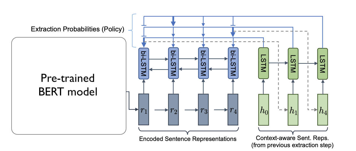
Figure 1: The image above shows the general architecture of the extractor.

This section describes the steps involved with deciding which sentences to extract.

BERT Embeddings

The first step of extraction is to represent all sentences as embeddings (left hand side of Figure 1). To do this, we use a pre-trained BERT model. The input to a BERT model can look like this:

“[CLS] A man in Florida was fined by police for indecent exposure in front of an elderly care home [SEP]”

The output embedding would look like this:

torch.tensor([[
	[0.9, 0.03, -0.4, …],
	[...]
	[0.04, -0.1, 0.3, …]
]])

In the above, each embedding row within the tensor corresponds to a word within the input. Additionally, the tokens “[CLS]” and “[SEP]” are pre/appended and their corresponding embeddings appear in the output tensor just like each word. The “[CLS]” is short for “classifier” and marks the start of a sentence. The “[SEP]” token is short for “separator” and marks the end of a sentence

Why do we add these tokens? In addition to language modeling, BERT models are also trained for next sentence prediction (NSP). Given a pair of sentences, the BERT model is tasked to predict if the two sentences actually appear together within the source documents. For example:

“[CLS] A man in Florida was fined by police for indecent exposure in front of an elderly care home. [SEP] Penguins love to eat fish.”

“[CLS] A man in Florida was fined by police for indecent exposure in front of an elderly care home. [SEP] The man was arrested on 2PM Sunday Sept 27th and was found to be heavily influenced by drugs and alcohol.”

In the first example, the classifier embedding, once passed through a simple feed forward layer, would result in a low probability. The second would result in a high probability.

Although the classifier token was originally trained for NSP, in this approach, it has been repurposed to represent the entire sentence for the purpose of extraction. As a result, we are able to have an embedding for each sentence within a document.

LSTM

THe next step is to fine-tune the pre-trained BERT embeddings. This is step is shown in blue of Figure 1. Since BERT sentence embeddings are bi-directional in nature, they already capture the context of the words around it. However, in keeping with the original paper, sentence embeddings are passed through a bi-directional LSTM. This is arguably not necessary as one of the benefits of using a bi-directional LSTM is that it captures the context of the words around it.

NOTE: Moving forward, I will be mentioning the shape of tensors a lot as I always find it helpful when I learn anything related to neural networks!

The Bi-LSTM’s hidden states at each time step are used to represent new “fine-tuned” sentence embeddings. The input to the Bi-LSTM is of shape: (batch_size, n_sentences, bert_embedding_size) and the output is of shape: (batch_size, n_sentences, bi_lstm_hidden_size*2). The *2 is because the LSTM is bi-directional and we concatenate the hidden states from each direction.

bi_lstm_hidden_state, __ = self.bi_lstm(bert_sent_embeddings)

As a result, we’ve obtained an embedding of size bi_lstm_hidden_size*2 for each sentence within the article. To select the first sentence to extract, we will be using “attention” described in the next section.

Attention

Next, we use a second “pointer-LSTM”, shown in green in Figure 1, to calculate attention and start extracting sentences. To do this, we perform the following procedure:

1. Initialize input_embedding, h0, to be a randomized embedding of shape (batch_size, 1, fine_tuned_embedding_size*2).
2. Initialize init_hidden_cell_state to be an embedding filled with zeros of shape (batch_size, 1, fine_tuned_embedding_size*2). In hindsight, perhaps I should have used the Bi-LSTM’s hidden state of the last time step instead.

3. Use input_embedding and init_hidden_cell_state as inputs to the pointer-LSTM and obtain a new hidden_state of shape (batch_size, 1, fine_tuned_embedding_size*2).

    ptr_hidden_state, init_hidden_cell_state = self.ptr_lstm(input_embedding, init_hidden_cell_state)
   

4. Take the dot product between the new ptr_hidden_state and the all of the source document’s sentence embeddings, bi_lstm_hidden_state. The result of the dot product takes the shape of (batch_size, 1, n_sentences). Each of the values represent the amount of attention we should pay to each sentence embedding.

    attn_values = torch.bmm(ptr_hidden_state, bi_lstm_hidden_state.transpose(1, 2))
   

5. Take the attn_values calculated above and turn them into self_attn_weights by putting them through a softmax layer. This result maintains its shape of (batch_size, 1, n_sentences). These self_attn_weights represent how much “attention” should be paid to each of the source documents sentences.

    self_attn_weights = self.softmax(attn_values)
   

6. Obtain the weighted sum of all of the source document sentence embeddings in order to obtain a “context” embedding. To do this, we can take the dot product between the attention_weights and sentence embeddings. The resulting shape is (batch_size, 1, fine_tuned_embedding_size*2).

    context = torch.mm(self_attn_weights, bi_lstm_hidden_state)
   

7. Take the dot product between the context embedding and the source sentence embeddings to obtain an additional set of attention values of shape (batch_size, 1, n_sentence_words). Click here to watch a video by Yannic Kilcher for an explanation of why calcualte attention more than once.

    attn_values = torch.mm(context, bi_lstm_hidden_state.transpose(1, 2)
   

8. Calculate the extraction_probability by using a softmax layer and maintain the shape of (batch_size, 1, n_sentence_words)

    extraction_prob = self.softmax(attn_values)
   

9. Next, we retrieve the sentence embedding that has the highest extraction_probability and use that as the new input_embedding.

    ext_ent_idx = torch.argmax(extraction_prob)
    input_embedding = bi_lstm_hidden_state[0:1, ext_sent_idx:ext_sent_idx+1, :]
   

10. Return to step 3 until the number of extracted sentences matches the number of sentences extracted in the label. Note: The number of sentences to extract can be “learned” during the reinforcement learning portion. However, it is sufficient to extract the same number of sentences as found in the labels for now.

Put together, the algorithm looks like:

bi_lstm_hidden_state, __ = bi_lstm(bert_sent_embeddings)
input_embedding = init_sent_embedding.unsqueeze(0) 
init_hidden_cell_state = None
extraction_probs = list()

for i in range(n_ext_sents):
    # Obtain context
    ptr_hidden_state, init_hidden_cell_state = ptr_lstm(input_embedding, init_hidden_cell_state)
    attn_values = torch.bmm(ptr_hidden_state, bi_lstm_hidden_state.transpose(1, 2))
    self_attn_weights = softmax(attn_values)
    context = torch.bmm(self_attn_weights, bi_lstm_hidden_state)

    # Obtain extraction probability
    attn_values = torch.bmm(context, bi_lstm_hidden_state.transpose(1, 2))
    extraction_prob = softmax(attn_values)
    extraction_probs.append(extraction_prob)

    # Obtain next input embedding
    ext_sent_idx = torch.argmax(extraction_prob)
    input_embedding = bi_lstm_hidden_state[0:1, ext_sent_idx:ext_sent_idx+1, :]

Please click here for a jupyter notebook containing a minimum working example of this code.

Learning

In order to improve model parameters, we use the cross-entropy loss function:

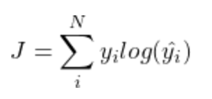
Using the output from step 8 in the previous section, we obtain an extraction probability for each sentence within the article. The extraction probability is plugged into the loss function as ŷ and we optimize using gradient descent to iteratively improve the weights of the following models:

• Bi-Directional LSTM network used to “fine tune” BERT embeddings
• Pointer LSTM network used to assign extraction probabilities

Conclusion

Here is a quick review regarding the key takeaways from this blogpost:

In this blogpost we have mentioned the steps of the overall summarization approach:

1. Choose which sentences to extract using BERT embeddings
2. Form an abstract summary from extracted sentences
3. Improve extraction and abstraction using reinforcement learning

Additionally, we have gone into depth on how sentences are chosen for extraction:

1. Convert each sentence within the article into a BERT embedding
2. Reduce the dimensionality of the BERT embeddings using a simple feed forward layer
3. Use a bi-directional LSTM model to further refine the sentence embeddings
4. Use a pointer LSTM model to assign an extraction probability to each sentence using attention
5. Improve the parameters of the two models using a cross-entropy loss function