Dungeons and Data

In this blog post, I apply reinforcement learning algorithms to a simple Dungeons and Dragons combat scenario. The code associated with this blog post can be seen in this github repo.

Combat Scenario Description

This section discusses the environment in which combat takes place.

As a first attempt, reinforcement learning was applied in a simple environment. The combat takes place in a 50ft x 50ft room and only involves two combatants:

1. Leotris:
   • Hit points: 25
   • Armor class: 16
   • Speed: 30ft
   • Shoot arrow attack:
     • 60 ft range
     • Hit bonus: +5
     • Damage dice: 1d12
     • Damage bonus: +3
   • Initial coordinates: (5, 5)
2. Strahd:
   • Hit points: 200
   • Armor class: 16
   • Speed: 30ft
   • Vampire bite attack:
     • 5 ft range
     • Hit bonus: +10
     • Damage dice: 3d12
     • Damage bonus: +10
   • Initial coordinates: (5, 10)

Each combatant, along with the attacks listed above, is allowed to take the following actions:

• MoveLeft: move left 5ft
• MoveRight: move right 5ft
• MoveDown: move down 5ft
• MoveUp: move up 5ft
• EndTurn: ends turn

Additionally, a “time limit” of 1500 actions was implemented. In other words, agents were permitted to take a maximum of 1500 actions within a single combat encounter.

Goals, Learning Environment, and Rewards

For this experiment, Leotris was assigned one of the RL algorithms described below while Strahd was assigned a Random strategy in which actions were chosen at random.

The scenario was purposefully set up such that Strahd had an obvious advantage. However, if Leotris is able learn to keep his distance from Strahd and use his ShootArrow attack, he should be able to win a considerable amount of the games.

The following are learning goals I envisioned for Leotris:

• Leotris out performs strategy of taking random actions.
• Leotris learns to deal damage. The challenge with this goal is that the agent must learn that it cannot just repeatedly take the ShootArrow action within the same turn. Instead, due to D&D combat rules, the agent must take the EndTurn action in between each ShootArrow usage if damage is to be done.
• Leotris learns to avoid damage. Leotris can only take damage from Strahd if they are within 5 ft of each other.

In order to accomplish the above goals, the agent’s “state” consists of the following:

1. Current hit points
2. Enemy hit points
3. Current x-coordinate
4. Current y-coordinate
5. Enemy x-coordinate
6. Enemy y-coordinate
7. Number of attacks used this turn
8. Remaining movement available this turn
9. Time limit remaining (as a percentage of the time limit)

Additionally, a reward of 5 was given if Leotris was the winner. Otherwise, a reward of 0 was given if Leotris had reached the “time limit” (1500 actions) or his hit points are reduced to zero.

Results and Discussion

Random

The figure below shows the result if both Strahd and Leotris are selecting actions at random.

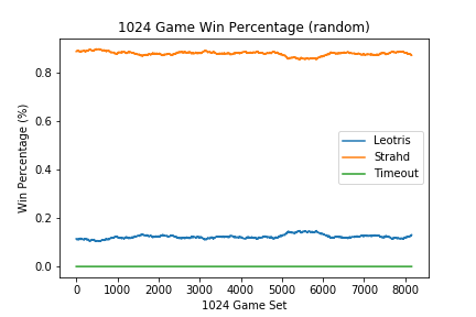
The above was used to evaluate whether goal 1 had been achieved.

Dueling Double Deep Q-Learning Network

The first RL algorithm I implemented was a vanilla DQN. However, after implenting it, I did not find immediate success. I then proceeded to add more “bells and whistles” and eventually arrived at a dueling double DQN. Below is a code snippet showing a portion of the dueling double DQN implementation used:

class DuelingNet(torch.nn.Module):
    def __init__(self, n_features, n_outputs, n_hidden_units):
        super(DuelingNet, self).__init__()
        self.layer_1 = torch.nn.Linear(n_features, n_hidden_units)

        self.value_layer_1 = torch.nn.Linear(n_hidden_units, n_hidden_units)
        self.value_layer_2 = torch.nn.Linear(n_hidden_units, 1)

        self.advantage_layer_1 = torch.nn.Linear(n_hidden_units, n_hidden_units)
        self.advantage_layer_2 = torch.nn.Linear(n_hidden_units, n_outputs)

        self.relu = torch.nn.ReLU()

    def forward(self, state):
        layer_1_output = self.layer_1(state)
        layer_1_output = self.relu(layer_1_output)

        value_output = self.value_layer_1(layer_1_output)
        value_output = self.relu(value_output)
        value_output = self.value_layer_2(value_output)

        advantage_output = self.advantage_layer_1(layer_1_output)
        advantage_output = self.relu(advantage_output)
        advantage_output = self.advantage_layer_2(advantage_output)

        q_output = value_output + advantage_output - advantage_output.mean(dim=1, keepdim=True)

        return q_output

When the above code was initially implemented, the follow results were achieved:

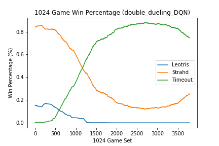
Similar results were observed for a vanilla DQN and double DQN. During training, the agent seemed to learn that the action ShootArrow was the best action to perform regardless of the current_state. Unfortunately, the agent would attempt to ShootArrow despite the fact that it had already used the action earlier within the same turn, which is against the rules. As a result, the action would be ignored and the agent would be prompted for its next action until the EndTurn action was chosen or the time limit was reached. The agent never learned when to take the EndTurn action consistently resulted a Timeout terminal state as observed in the plot above.

Although initial results did not show evidence that a reasonable strategy had been learned, the agent began to exhibit improved performance with a some key adjustments:

1. Reducing Learning rate α: Perhaps the most important adjustment that had to be made was optimizing the learning rate α. With too large of a learning rate, the agent could not “escape” areas of suboptimal strategies within the parameter space.
2. Reducing ϵ-exploration decay rate: The linearly decaying ϵ-greedy exploration strategy was implemented such that the agent started with an ϵ-exploration probability of 90% which decayed linearly to 5% over 50,000 actions. That is to say, at the beginning stages of exploration, the agent would take the action believed to be optimal 10% of the time. The remaining 90% of the time, the agent would “explore” by taking a random action. The ϵ-value would decay linearly down to a 5% exploration. This was far too fast of a decay rate and the agent failed to explore enough in order to learn a reasonable strategy.
3. Making rewards less sparse: By only providing a reward for achieving a victory, the training objective was made more difficult. To address this, rewards were changed such that the agent was rewarded every time it did damage. This helped a great deal with the agent even learning to alter between ShootArrow and EndTurn. Although this was a great quick fix, I decided to return the reward structure back to the original as I was more interested in a sparser reward setting.
4. Avoiding catastrophic forgetting: Looking at this stack exchange post, the user is asking why DQNs sometimes train themselves out of desired behavior. I observed this happening when the agent was able to establish a reasonable strategy at the terminal ϵ-exploration of 5%, but if it was left to train longer, performance would eventually degrade. To combat this, it was suggested to decrease the learning rate and use prioritized experience replay. This seemed to help. Another suggestion was to keep experiences from early stages of exploration within memory. I have not tried this one yet.

Once the above were adjusted, the agent was able to learn a reasonable strategy which exhibited the following results:

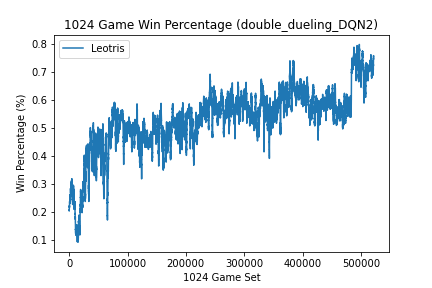
(I cannot stress how happy I was to see these results. Although the scenario was relatively simplisitic and seemingly not difficult, after countless attempts of failed agents, this was a sight for extremely sore eyes.)

Proximal Policy Iteration (PPO)

Here is a code snippet showing the PPO implementation that was used:

class ActorCritic(torch.nn.Module):
    def __init__(self, n_features, n_outputs, n_hidden_units):
        """
        :param n_features:
        :param n_outputs:
        :param n_hidden_units:
        """
        super(ActorCritic, self).__init__()

        # Actor
        self.actor_layer = torch.nn.Sequential(
            torch.nn.Linear(n_features, n_hidden_units),
            torch.nn.ReLU(),
            torch.nn.Linear(n_hidden_units, n_outputs),
            torch.nn.Softmax(dim=-1)
        )

        # Critic
        self.critic_layer = torch.nn.Sequential(
            torch.nn.Linear(n_features, n_hidden_units),
            torch.nn.ReLU(),
            torch.nn.Linear(n_hidden_units, 1)
        )

    def forward(self, state):
        actor_output = self.actor_layer(state)
        value = self.critic_layer(state)
        dist = Categorical(actor_output)

        return dist, value

    def evaluate(self, state, action_index):
        actor_output = self.actor_layer(state)
        dist = Categorical(actor_output)
        entropy = dist.entropy().mean()
        log_probs = dist.log_prob(action_index.view(-1))
        value = self.critic_layer(state)

        return log_probs, value, entropy

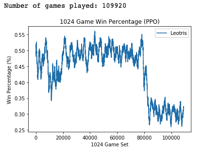
With the above implementation of PPO a reasonable strategy was learned:

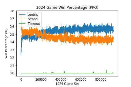
I believe that there were a couple contributing factors in obtaining these results. Again it was vital that the learning rate be sufficiently small (α=1e-5). With a larger learning rate of (α=1e-3), the following results were observed:

Similar to the dueling double DQN, the PPO agent seems to have gotten into a parameter space in which it could not recover from if α was too large.

I found that the PPO agent was not as sensitive to hyper parameter tuning and worked better out of the box. Perhaps the largest contributing factors is the fact that the agent did not use an epsilon greedy like exploration strategy. Instead, PPO agents select actions stochastically by nature and does not require an explicit exploration strategy. As a result, it was less likely to get “stuck” in a bad area because it would naturally revert back to a higher exploration mode.

Although I was not able achieve as high of a win percentage as the dueling double DQN, I don’t think it that this is indicative of the potential of PPO. I spent a lot more time adjusting hyper parameters and adding bells and whistles for DQNs. I believe if the PPO network was made deeper and the learning rate was properly tuned, it would be able to match the performance of the DQN.

Conclusion

Here are some key takeaways I gained from this project:

1. Reinforcement learning can take a long time. When I first started, I would often stop training an agent prematurely if it hadn’t shown early signs of success or saw if there was dip in performance. However, I later learned that agents could overcome areas of low performance and even surpass previous performance highs.
2. Learning rate is almost always the most imporant hyper parameter.
3. Implement algorithms in small and simple scenarios first. This helps immensely with debugging and speeding iteration cycles.
4. It’s a good idea to make your solution fast and scalable. This is an area I neglected and a large source of frustration for me. Operating on a slow iteration cycle was painful with instances in which I waited for days for the agent to learn a reasonable strategy only to find out there was a bug or that I wanted to adjust a hyperparameter. If I had made my solution more scalable, I could have cut down on the time waiting around.
5. Don’t let perfection get in the way of progress. Is my code a piece of low quality? Yes. Did I learn a lot by doing this? Yes